QMRI Challenge ISMRM 2024 - \(T_1\) mapping

In the 2024 ISMRM QMRI Challenge, the goal is to estimate \(T_1\) maps from a set of inversion recovery images. The dataset consists of images obtained at 10 different inversion times using a turbo spin echo sequence. Each inversion time is saved in a separate DICOM file. In order to obtain a \(T_1\) map, we are going to:

• download the data from Zenodo

• read in the DICOM files (one for each inversion time) and combine them in an IData object

• define a signal model and data loss (mean-squared error) function

• find good starting values for each pixel

• carry out a fit using ADAM from PyTorch

Get data from Zenodo

import tempfile
import zipfile
from pathlib import Path

import zenodo_get

dataset = '10868350'

tmp = tempfile.TemporaryDirectory()  # RAII, automatically cleaned up
data_folder = Path(tmp.name)
zenodo_get.zenodo_get([dataset, '-r', 5, '-o', data_folder])  # r: retries
with zipfile.ZipFile(data_folder / Path('T1 IR.zip'), 'r') as zip_ref:
    zip_ref.extractall(data_folder)

Create image data (IData) object with different inversion times

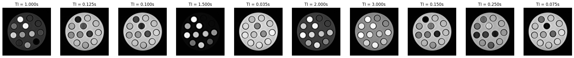
We read in the DICOM files and combine them in an IData object. The inversion times are stored in the DICOM files are available in the header of the IData object.

import mrpro

ti_dicom_files = data_folder.glob('**/*.dcm')
idata_multi_ti = mrpro.data.IData.from_dicom_files(ti_dicom_files)

if idata_multi_ti.header.ti is None:
    raise ValueError('Inversion times need to be defined in the DICOM files.')

Show plotting details Hide code cell content

import matplotlib.pyplot as plt
import torch


def show_images(*images: torch.Tensor, titles: list[str] | None = None) -> None:
    """Plot images."""
    n_images = len(images)
    _, axes = plt.subplots(1, n_images, squeeze=False, figsize=(n_images * 3, 3))
    for i in range(n_images):
        axes[0][i].imshow(images[i], cmap='gray')
        axes[0][i].axis('off')
        if titles:
            axes[0][i].set_title(titles[i])
    plt.show()

# Let's have a look at some of the images
show_images(
    *idata_multi_ti.data[:, 0, 0].abs(),
    titles=[f'TI = {ti:.3f}s' for ti in idata_multi_ti.header.ti.squeeze()],
)

Signal model and loss function

We use the model \(q\)

\(q(TI) = M_0 (1 - e^{-TI/T_1})\)

with the equilibrium magnetization \(M_0\), the inversion time \(TI\), and \(T_1\). We have to keep in mind that the DICOM images only contain the magnitude of the signal. Therefore, we need \(|q(TI)|\):

model = mrpro.operators.MagnitudeOp() @ mrpro.operators.models.InversionRecovery(ti=idata_multi_ti.header.ti)

As a loss function for the optimizer, we calculate the mean-squared error between the image data \(x\) and our signal model \(q\).

mse = mrpro.operators.functionals.MSE(idata_multi_ti.data.abs())

Now we can simply combine the two into a functional to solve

\( \min_{M_0, T_1} || |q(M_0, T_1, TI)| - x||_2^2\)

functional = mse @ model

Starting values for the fit

We are trying to minimize a non-linear function \(q\). There is no guarantee that we reach the global minimum, but we can end up in a local minimum.

To increase our chances of reaching the global minimum, we can ensure that our starting values are already close to the global minimum. We need a good starting point for each pixel.

One option to get a good starting point is to calculate the signal curves for a range of \(T_1\) values and then check for each pixel which of these signal curves fits best. This is similar to what is done for MR Fingerprinting. So we are going to:

• define a list of realistic \(T_1\) values (we call this a dictionary of \(T_1\) values)

• calculate the signal curves corresponding to each of these \(T_1\) values

• compare the signal curves to the signals of each voxel (we use the maximum of the dot-product as a metric of how well the signals fit to each other)

# Define 100 T1 values between 0.1 and 3.0 s
t1_dictionary = torch.linspace(0.1, 3.0, 100)

# Calculate the signal corresponding to each of these T1 values. We set M0 to 1, but this is arbitrary because M0 is
# just a scaling factor and we are going to normalize the signal curves.
(signal_dictionary,) = model(torch.ones(1), t1_dictionary)
signal_dictionary = signal_dictionary.to(dtype=torch.complex64)
signal_dictionary /= torch.linalg.vector_norm(signal_dictionary, dim=0)

# Calculate the dot-product and select for each voxel the T1 values that correspond to the maximum of the dot-product
import einops

dot_product = einops.einsum(
    idata_multi_ti.data,
    signal_dictionary,
    'ti ..., ti t1 -> t1 ...',
)
idx_best_match = dot_product.abs().argmax(dim=0)
t1_start = t1_dictionary[idx_best_match]

The maximum absolute value observed is a good approximation for \(M_0\)

m0_start = idata_multi_ti.data.abs().amax(dim=0)

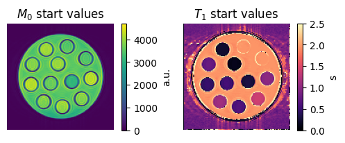
Visualize the starting values

Let’s have a look at the starting values for \(M_0\) and \(T_1\):

fig, axes = plt.subplots(1, 2, figsize=(6, 2), squeeze=False)

im = axes[0, 0].imshow(m0_start[0, 0])
axes[0, 0].set_title('$M_0$ start values')
axes[0, 0].set_axis_off()
fig.colorbar(im, ax=axes[0, 0], label='a.u.')

im = axes[0, 1].imshow(t1_start[0, 0], vmin=0, vmax=2.5, cmap='magma')
axes[0, 1].set_title('$T_1$ start values')
axes[0, 1].set_axis_off()
fig.colorbar(im, ax=axes[0, 1], label='s')

plt.show()

Carry out fit

We are now ready to carry out the fit. We are going to use the adam optimizer. If there is a GPU available, we can use it ny moving both the data and the model to the GPU.

# Move initial values and model to GPU if available
if torch.cuda.is_available():
    print('Using GPU')
    functional.cuda()
    m0_start = m0_start.cuda()
    t1_start = t1_start.cuda()

# Hyperparameters for optimizer
max_iter = 2000
lr = 1e-1

# Run optimization
result = mrpro.algorithms.optimizers.adam(functional, [m0_start, t1_start], max_iter=max_iter, lr=lr)
m0, t1 = (p.detach().cpu() for p in result)

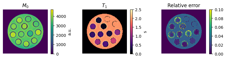
Visualize the final results

To get an impression of how well the fit has worked, we are going to calculate the relative error between

\(E_{relative} = \sum_{TI}\frac{|(q(M_0, T_1, TI) - x)|}{|x|}\)

on a voxel-by-voxel basis We also mask out the background by thresholding on \(M_0\).

error = model(m0, t1)[0] - idata_multi_ti.data
relative_absolute_error = error.abs().sum(dim=0) / (idata_multi_ti.data.abs().sum(dim=0) + 1e-9)

mask = torch.isnan(t1) | (m0 < 500)
m0[mask] = 0
t1[mask] = 0
relative_absolute_error[mask] = 0

fig, axes = plt.subplots(1, 3, figsize=(10, 2), squeeze=False)
im = axes[0, 0].imshow(m0[0, 0])
axes[0, 0].set_title('$M_0$')
axes[0, 0].set_axis_off()
fig.colorbar(im, ax=axes[0, 0], label='a.u.')

im = axes[0, 1].imshow(t1[0, 0], vmin=0, vmax=2.5, cmap='magma')
axes[0, 1].set_title('$T_1$')
axes[0, 1].set_axis_off()
fig.colorbar(im, ax=axes[0, 1], label='s')

im = axes[0, 2].imshow(relative_absolute_error[0, 0], vmin=0, vmax=0.1)
axes[0, 2].set_title('Relative error')
axes[0, 2].set_axis_off()
fig.colorbar(im, ax=axes[0, 2])

plt.show()

Next steps

The 2024 ISMRM QMRI Challenge also included the estimation of \(T_2^*\) maps from multi-echo data. You can find the the data on zenodo in record 10868361 as T2star.zip You can download and unpack it using the same method as above.

As a signal model \(q\) you can use MonoExponentialDecay describing the signal decay as \(q(TE) = M_0 e^{-TE/T_2^*}\) with the equilibrium magnetization \(M_0\), the echo time \(TE\), and \(T_2^*\).
Give it a try and see if you can obtain good \(T_2^*\) maps!

Note

The echo times \(TE\) can be found in IData.header.te. A good starting value for \(M_0\) is the signal at the shortest echo time. A good starting value for \(T_2^*\) is 20 ms.