Iterative SENSE reconstruction of 2D golden angle radial data

Here we use an iterative reconstruction method reconstruct images from ISMRMRD 2D radial data.

We use the IterativeSENSEReconstruction class to reconstruct images by solving the following reconstruction problem:

Let’s assume we have obtained the k-space data \(y\) from an image \(x\) with an acquisition model (Fourier transforms, coil sensitivity maps…) \(A\) then we can formulate the forward problem as:

\( y = Ax + n \)

where \(n\) describes complex Gaussian noise. The image \(x\) can be obtained by minimizing the functional \(F\)

\( F(x) = ||W^{\frac{1}{2}}(Ax - y)||_2^2 \)

where \(W^\frac{1}{2}\) is the square root of the density compensation function (which corresponds to a diagonal operator) used to weight the loss.

Setting the derivative of the functional \(F\) to zero and rearranging yields

\( A^H W A x = A^H W y\)

which is a linear system \(Hx = b\) that needs to be solved for \(x\). This is done using the conjugate gradient method.

Using IterativeSENSEReconstruction

First, we demonstrate the use of IterativeSENSEReconstruction, before we peek behind the scenes and implement the reconstruction manually.

Read-in the raw data

We read the raw k-space data and the trajectory from the ISMRMRD file (see Different ways to obtain the trajectory for more information on the trajectory calculation). Our example data contains three datasets:

• radial2D_402spokes_golden_angle_with_traj.h5 with 402 spokes

• radial2D_96spokes_golden_angle_with_traj.h5 with 96 spokes

• radial2D_24spokes_golden_angle_with_traj.h5 with 24 spokes

We use the 402 spokes dataset for the reconstruction.

Show download details Hide code cell content

# ### Download raw data from Zenodo
import tempfile
from pathlib import Path

import zenodo_get

dataset = '14617082'

tmp = tempfile.TemporaryDirectory()  # RAII, automatically cleaned up
data_folder = Path(tmp.name)
zenodo_get.zenodo_get([dataset, '-r', 5, '-o', data_folder])  # r: retries

import mrpro

trajectory_calculator = mrpro.data.traj_calculators.KTrajectoryIsmrmrd()
kdata = mrpro.data.KData.from_file(data_folder / 'radial2D_402spokes_golden_angle_with_traj.h5', trajectory_calculator)

Direct reconstruction for comparison

For comparison, we first can carry out a direct reconstruction using the DirectReconstruction class. See also Direct reconstruction of 2D golden angle radial data.

direct_reconstruction = mrpro.algorithms.reconstruction.DirectReconstruction(kdata)
img_direct = direct_reconstruction(kdata)

Setting up the iterative SENSE reconstruction

Now let’s use the IterativeSENSEReconstruction class to reconstruct the image using the iterative SENSE algorithm.

We first set up the reconstruction. Here, we reuse the the Fourier operator, the DCFs and the coil sensitivity maps from direct_reconstruction. We use early stopping after 4 iterations by setting n_iterations.

Note

When settings up the reconstruction can also just provide the KData and let IterativeSENSEReconstruction figure out the Fourier operator, estimate the coil sensitivity maps, and choose a density weighting.
We can also provide KData and some information, such as the sensitivity maps. In that case, the reconstruction will fill in the missing information based on the KData object.

iterative_sense_reconstruction = mrpro.algorithms.reconstruction.IterativeSENSEReconstruction(
    fourier_op=direct_reconstruction.fourier_op,
    csm=direct_reconstruction.csm,
    dcf=direct_reconstruction.dcf,
    n_iterations=4,
)

Run the reconstruction

We now run the reconstruction using iterative_sense_reconstruction object. We just need to pass the k-space data and obtain the reconstructed image as IData object.

img = iterative_sense_reconstruction(kdata)

Behind the scenes

We now peek behind the scenes to see how the iterative SENSE reconstruction is implemented. We perform all steps IterativeSENSEReconstruction does when initialized with only an KData object, i.e., we need to set up a Fourier operator, estimate coil sensitivity maps, and the density weighting. without reusing any thing from ``direct_reconstruction```.

Set up density compensation operator \(W\)

We create a density compensation operator \(W\) for weighting the loss. We use Voronoi tessellation of the trajectory to calculate the DcfData.

Note

Using a weighted loss in iterative SENSE is not necessary, and there has been some discussion about the benefits and drawbacks. Currently, the iterative SENSE reconstruction in mrpro uses a weighted loss. This might chang in the future.

dcf_operator = mrpro.data.DcfData.from_traj_voronoi(kdata.traj).as_operator()

Set up the acquisition model \(A\)

We need FourierOp and SensitivityOp operators to set up the acquisition model \(A\). The Fourier operator is created from the trajectory and header information in kdata:

fourier_operator = mrpro.operators.FourierOp(
    traj=kdata.traj,
    recon_matrix=kdata.header.recon_matrix,
    encoding_matrix=kdata.header.encoding_matrix,
)

To estimate the coil sensitivity maps, we first calculate the coil-wise images from the k-space data and then estimate the coil sensitivity maps using the Walsh method:

img_coilwise = mrpro.data.IData.from_tensor_and_kheader(*fourier_operator.H(*dcf_operator(kdata.data)), kdata.header)
csm_data = mrpro.data.CsmData.from_idata_walsh(img_coilwise)
csm_operator = csm_data.as_operator()

Now we can set up the acquisition operator \(A\) by composing the Fourier operator and the coil sensitivity maps operator using @.

acquisition_operator = fourier_operator @ csm_operator

Calculate the right-hand-side of the linear system

Next, we need to calculate \(b = A^H W y\).

(right_hand_side,) = (acquisition_operator.H @ dcf_operator)(kdata.data)

Set-up the linear self-adjoint operator \(H\)

We setup \(H = A^H W A\), using the dcf_operator and acquisition_operator.

operator = acquisition_operator.H @ dcf_operator @ acquisition_operator

Run conjugate gradient

Finally, we solve the linear system \(Hx = b\) using the conjugate gradient method. Again, we use early stopping after 4 iterations. Instead, we could also use a tolerance to stop the iterations when the residual is below a certain threshold.

img_manual = mrpro.algorithms.optimizers.cg(
    operator, right_hand_side, initial_value=right_hand_side, max_iterations=4, tolerance=0.0
)

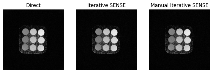
Display the results

We can now compare the results of the iterative SENSE reconstruction with the direct reconstruction. Both versions, the one using the IterativeSENSEReconstruction class and the manual implementation should result in identical images.

Show plotting details Hide code cell content

import matplotlib.pyplot as plt
import torch


def show_images(*images: torch.Tensor, titles: list[str] | None = None) -> None:
    """Plot images."""
    n_images = len(images)
    _, axes = plt.subplots(1, n_images, squeeze=False, figsize=(n_images * 3, 3))
    for i in range(n_images):
        axes[0][i].imshow(images[i], cmap='gray')
        axes[0][i].axis('off')
        if titles:
            axes[0][i].set_title(titles[i])
    plt.show()

show_images(
    img_direct.rss()[0, 0],
    img.rss()[0, 0],
    img_manual.abs()[0, 0, 0],
    titles=['Direct', 'Iterative SENSE', 'Manual Iterative SENSE'],
)

Check for equal results

Finally, we check if two images are really identical.

# If the assert statement did not raise an exception, the results are equal.
assert torch.allclose(img.data, img_manual)

Next steps

We can also reconstruct undersampled data: You can replace the filename above to use a dataset with fewer spokes to try it out.
If you want to see how to include a regularization term in the optimization problem, see the example in Regularized iterative SENSE reconstruction of 2D golden angle radial data.