![]()
Direct reconstruction of 2D golden angle radial data
Here we use the DirectReconstruction class to perform a basic reconstruction of
2D radial data.
A direct reconstruction uses the density compensated adjoint of the acquisition operator to obtain the images.
Using DirectReconstruction
We use the DirectReconstruction class to reconstruct images from 2D radial data.
DirectReconstruction estimates sensitivity maps, density compensation factors, etc.
and performs an adjoint Fourier transform.
This the simplest reconstruction method in our high-level interface to the reconstruction pipeline.
Load the data
We load in the Data from the ISMRMRD file. We want use the trajectory that is stored also stored the ISMRMRD file.
This can be done by passing a KTrajectoryIsmrmrd object to
from_file when loading creating the KData.
Show download details
# Download raw data from Zenodo
import tempfile
from pathlib import Path

import zenodo_get

dataset = '14617082'

tmp = tempfile.TemporaryDirectory()  # RAII, automatically cleaned up
data_folder = Path(tmp.name)
zenodo_get.zenodo_get([dataset, '-r', 5, '-o', data_folder])  # r: retries
import mrpro
import torch

trajectory_calculator = mrpro.data.traj_calculators.KTrajectoryIsmrmrd()
kdata = mrpro.data.KData.from_file(data_folder / 'radial2D_402spokes_golden_angle_with_traj.h5', trajectory_calculator)
Setup the DirectReconstruction instance
We create a DirectReconstruction and supply kdata.
DirectReconstruction uses the information in kdata to
setup a Fourier transfrm, density compensation factors, and estimate coil sensitivity maps.
(See the Behind the scenes section for more details.)
Note
You can also directly set the Fourier operator, coil sensitivity maps, density compensation factors, etc. of the reconstruction instance.
reconstruction = mrpro.algorithms.reconstruction.DirectReconstruction(kdata)
Perform the reconstruction
The reconstruction is performed by calling the passing the k-space data.
Note
Often, the data used to obtain the meta data for constructing the reconstruction instance is the same as the data passed to the reconstruction. But you can also different to create the coil sensitivity maps, dcf, etc. than the data that is passed to the reconstruction.
img = reconstruction(kdata)
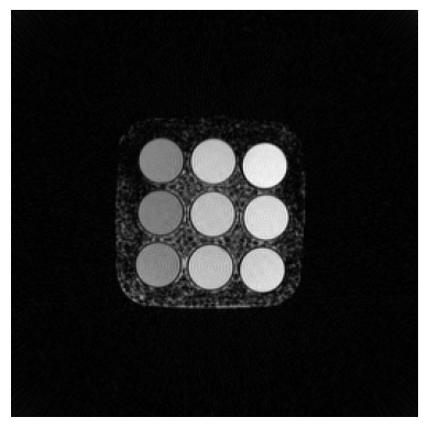
Display the reconstructed image
We now got in IData object containing a header and the image tensor.
We display the reconstructed image using matplotlib.
import matplotlib.pyplot as plt

# If there are multiple slices, ..., only the first one is selected
first_img = img.rss()[0, 0]  #  images, z, y, x
plt.imshow(first_img, cmap='gray')
plt.axis('off')
plt.show()
Behind the scenes
We now peek behind the scenes to see what happens in the DirectReconstruction
class, and perform all steps manually:
Calculate density compensation factors
Setup Fourier operator
Obtain coil-wise images
Calculate coil sensitivity maps
Perform direct reconstruction
Calculate density compensation using the trajectory
We use a Voronoi tessellation of the trajectory to calculate the DcfData and obtain
a DensityCompensationOp operator.
dcf_operator = mrpro.data.DcfData.from_traj_voronoi(kdata.traj).as_operator()
Setup Fourier Operator
Next, we create the Fourier operator. We can just pass the kdata object to the constructor of the
FourierOp, and the trajectory and header information is used to create the operator. We want the
to use the adjoint density compensated Fourier operator, so we perform a composition with dcf_operator
and use the H property of the operator to obtain its adjoint.
fourier_operator = dcf_operator @ mrpro.operators.FourierOp.from_kdata(kdata)
adjoint_operator = fourier_operator.H
Calculate coil sensitivity maps
Coil sensitivity maps are calculated using the walsh method (See CsmData for other available methods).
We first need to calculate the coil-wise images, which are then used to calculate the coil sensitivity maps.
img_coilwise = mrpro.data.IData.from_tensor_and_kheader(*adjoint_operator(kdata.data), kdata.header)
csm_operator = mrpro.data.CsmData.from_idata_walsh(img_coilwise).as_operator()
Perform Direct Reconstruction
Finally, the direct reconstruction is performed and an IData object with the reconstructed
image is returned. We update the adjoint_operator to also include the coil sensitivity maps, thus
performing the coil combination.
adjoint_operator = (fourier_operator @ csm_operator).H
img_manual = mrpro.data.IData.from_tensor_and_kheader(*adjoint_operator(kdata.data), kdata.header)
Further behind the scenes
There is also a even more manual way to perform the direct reconstruction. We can set up the Fourier operator by passing the trajectory and matrix sizes.
fourier_operator = mrpro.operators.FourierOp(
    recon_matrix=kdata.header.recon_matrix,
    encoding_matrix=kdata.header.encoding_matrix,
    traj=kdata.traj,
)
We can call one of the algorithms in mrpro.algorithms.dcf to calculate the density compensation factors.
kykx = torch.stack((kdata.traj.ky[0, 0], kdata.traj.kx[0, 0]))
dcf_tensor = mrpro.algorithms.dcf.dcf_2d3d_voronoi(kykx)
We use these DCFs to weight the k-space data before performing the adjoint Fourier transform. We can also call
adjoint on the Fourier operator instead of obtaining an adjoint operator.
(img_tensor_coilwise,) = fourier_operator.adjoint(dcf_tensor * kdata.data)
Next, we calculate the coil sensitivity maps by using one of the algorithms in mrpro.algorithms.csm and set
up a SensitivityOp operator.
csm_data = mrpro.algorithms.csm.walsh(img_tensor_coilwise[0], smoothing_width=5)
csm_operator = mrpro.operators.SensitivityOp(csm_data)
Finally, we perform the coil combination of the coil-wise images and obtain final images.
(img_tensor_coilcombined,) = csm_operator.adjoint(img_tensor_coilwise)
img_more_manual = mrpro.data.IData.from_tensor_and_kheader(img_tensor_coilcombined, kdata.header)
Check for equal results
The 3 versions result should in the same image data.
# If the assert statement did not raise an exception, the results are equal.
torch.testing.assert_close(img.data, img_manual.data)
torch.testing.assert_close(img.data, img_more_manual.data, atol=1e-4, rtol=1e-4)