Basics of MRpro and Cartesian reconstructions

Here, we are going to have a look at a few basics of MRpro and reconstruct data acquired with a Cartesian sampling pattern.

Overview

In this notebook, we are going to explore the KData object and the included header parameters. We will then use a FFT-operator in order to reconstruct data acquired with a Cartesian sampling scheme. We will also reconstruct data acquired on a Cartesian grid but with partial echo and partial Fourier acceleration. Finally, we will reconstruct a Cartesian scan with regular undersampling.

Show download details Hide code cell content

# Get the raw data from zenodo
import tempfile
from pathlib import Path

import zenodo_get

dataset = '14173489'

tmp = tempfile.TemporaryDirectory()  # RAII, automatically cleaned up
data_folder = Path(tmp.name)
zenodo_get.zenodo_get([dataset, '-r', 5, '-o', data_folder])  # r: retries

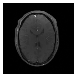
We have three different scans obtained from the same object with the same FOV and resolution, saved as ISMRMRD raw data files (*.mrd or *.h5):

• cart_t1.mrd is a fully sampled Cartesian acquisition

• cart_t1_msense_integrated.mrd is accelerated using regular undersampling and self-calibrated SENSE

• cart_t1_partial_echo_partial_fourier.mrd is accelerated using partial echo and partial Fourier

Read in raw data and explore header

To read in an ISMRMRD file, we can simply pass on the file name to a KData object. Additionally, we need to provide information about the trajectory. In MRpro, this is done using trajectory calculators. These are functions that calculate the trajectory based on the acquisition information and additional parameters provided to the calculators (e.g. the angular step for a radial acquisition).

In this case, we have a Cartesian acquisition. This means that we only need to provide a Cartesian trajectory calculator KTrajectoryCartesian without any further parameters.

See Different ways to obtain the trajectory for more information about different ways to define the trajectory.

import mrpro

kdata = mrpro.data.KData.from_file(
    data_folder / 'cart_t1.mrd',
    mrpro.data.traj_calculators.KTrajectoryCartesian(),
)

Now we can explore this data object. Simply printing kdata gives us a basic overview of the KData object.

print(kdata)

KData with shape [1, 16, 1, 256, 512] and dtype torch.complex64
Device: cpu
KTrajectory with shape: kz=[1, 1, 1, 1], ky=[  1,   1, 256,   1], kx=[  1,   1,   1, 512]
FOV [m]: z=0.004, y=0.256, x=0.512
TE [s]: [0.0029]
TI [s]: [0.3000]
Flip angle [rad]: None
Encoding matrix: z=1, y=256, x=512 
Recon matrix: z=1, y=256, x=256

We can also have a look at more specific header information like the 1H Lamor frequency

print('Lamor Frequency:', kdata.header.lamor_frequency_proton)

Lamor Frequency: 123252558

Reconstruction of fully sampled acquisition

For the reconstruction of a fully sampled Cartesian acquisition, we can either use a general FourierOp or manually set up a Fast Fourier Transform (FFT). For demonstration purposes, we first show the manual approach.

Note

Most of the time, you will use the FourierOp operator, which automatically takes care of choosing whether to use a FFT or a non-uniform FFT (NUFFT) based on the trajectory. It optionally can be created from a KData object without any further information.

Let’s create an FFT-operator FastFourierOp and apply it to our KData object. Please note that all MRpro operator work on PyTorch tensors and not on the MRpro objects directly. Therefore, we have to call the operator on kdata.data. One other important property of MRpro operators is that they always return a tuple of PyTorch tensors, even if the output is only a single tensor. This is why we use the (img,) syntax below.

fft_op = mrpro.operators.FastFourierOp(dim=(-2, -1))
(img,) = fft_op.adjoint(kdata.data)

Let’s have a look at the shape of the obtained tensor.

print('Shape:', img.shape)

Shape: torch.Size([1, 16, 1, 256, 512])

We can see that the second dimension, which is the coil dimension, is 16. This means we still have a coil resolved dataset (i.e. one image for each coil element). We can use a simply root-sum-of-squares approach to combine them into one. Later, we will do something a bit more sophisticated. We can also see that the x-dimension is 512. This is because in MRI we commonly oversample the readout direction by a factor 2 leading to a FOV twice as large as we actually need. We can either remove this oversampling along the readout direction or we can simply tell the FastFourierOp to crop the image by providing the correct output matrix size recon_matrix.

# Create FFT-operator with correct output matrix size
fft_op = mrpro.operators.FastFourierOp(
    dim=(-2, -1),
    recon_matrix=kdata.header.recon_matrix,
    encoding_matrix=kdata.header.encoding_matrix,
)

(img,) = fft_op.adjoint(kdata.data)
print('Shape:', img.shape)

Shape: torch.Size([1, 16, 1, 256, 256])

Now, we have an image which is 256 x 256 voxel as we would expect. Let’s combine the data from the different receiver coils using root-sum-of-squares and then display the image. Note that we usually index from behind in MRpro (i.e. -1 for the last, -4 for the fourth last (coil) dimension) to allow for more than one ‘other’ dimension.

Show plotting details Hide code cell content

import matplotlib.pyplot as plt
import torch


def show_images(*images: torch.Tensor, titles: list[str] | None = None) -> None:
    """Plot images."""
    n_images = len(images)
    _, axes = plt.subplots(1, n_images, squeeze=False, figsize=(n_images * 3, 3))
    for i in range(n_images):
        axes[0][i].imshow(images[i], cmap='gray')
        axes[0][i].axis('off')
        if titles:
            axes[0][i].set_title(titles[i])
    plt.show()

# Combine data from different coils and show magnitude image
magnitude_fully_sampled = img.abs().square().sum(dim=-4).sqrt().squeeze()
show_images(magnitude_fully_sampled)

Great! That was very easy! Let’s try to reconstruct the next dataset.

Reconstruction of acquisition with partial echo and partial Fourier

# Read in the data
kdata_pe_pf = mrpro.data.KData.from_file(
    data_folder / 'cart_t1_partial_echo_partial_fourier.mrd',
    mrpro.data.traj_calculators.KTrajectoryCartesian(),
)

# Create FFT-operator with correct output matrix size
fft_op = mrpro.operators.FastFourierOp(
    dim=(-2, -1),
    recon_matrix=kdata.header.recon_matrix,
    encoding_matrix=kdata.header.encoding_matrix,
)

# Reconstruct coil resolved image(s)
(img_pe_pf,) = fft_op.adjoint(kdata_pe_pf.data)

# Combine data from different coils using root-sum-of-squares
magnitude_pe_pf = img_pe_pf.abs().square().sum(dim=-4).sqrt().squeeze()

# Plot both images
show_images(magnitude_fully_sampled, magnitude_pe_pf, titles=['fully sampled', 'PF & PE'])

Well, we got an image, but when we compare it to the previous result, it seems like the head has shrunk. Since that’s extremely unlikely, there’s probably a mistake in our reconstruction.

Let’s step back and check out the trajectories for both scans.

print(kdata.traj)

KTrajectory with shape: kz=[1, 1, 1, 1], ky=[  1,   1, 256,   1], kx=[  1,   1,   1, 512]

We see that the trajectory has kz, ky, and kx components. kx and ky only vary along one dimension.

Note

This is because MRpro saves meta data such as trajectories in an efficient way, where dimensions in which the data does not change are often collapsed. The original shape can be obtained by broadcasting.

To get the full trajectory as a tensor, we can also just call as_tensor():

# Plot the fully sampled trajectory (in blue)
full_kz, full_ky, full_kx = kdata.traj.as_tensor()
plt.plot(full_ky[0, 0].flatten(), full_kx[0, 0].flatten(), 'ob')

# Plot the partial echo and partial Fourier trajectory (in red)
full_kz, full_ky, full_kx = kdata_pe_pf.traj.as_tensor()
plt.plot(full_ky[0, 0].flatten(), full_kx[0, 0].flatten(), '+r')

plt.show()

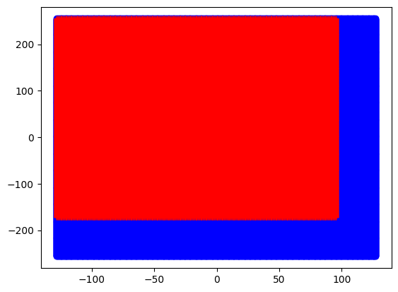
We see that for the fully sampled acquisition, the k-space is covered symmetrically from -256 to 255 along the readout direction and from -128 to 127 along the phase encoding direction. For the acquisition with partial Fourier and partial echo acceleration, this is of course not the case and the k-space is asymmetrical.

Our FFT-operator does not know about this and simply assumes that the acquisition is symmetric and any difference between encoding and recon matrix needs to be zero-padded symmetrically.

To take the asymmetric acquisition into account and sort the data correctly into a matrix where we can apply the FFT-operator to, we have got the CartesianSamplingOp in MRpro. This operator performs sorting based on the k-space trajectory and the dimensions of the encoding k-space.

Let’s try it out!

cart_sampling_op = mrpro.operators.CartesianSamplingOp(
    encoding_matrix=kdata_pe_pf.header.encoding_matrix, traj=kdata_pe_pf.traj
)

Now, we first apply the adjoint CartesianSamplingOp and then call the adjoint FFT-operator.

(img_pe_pf,) = fft_op.adjoint(cart_sampling_op.adjoint(kdata_pe_pf.data)[0])
magnitude_pe_pf = img_pe_pf.abs().square().sum(dim=-4).sqrt().squeeze()

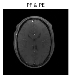
show_images(magnitude_fully_sampled, magnitude_pe_pf, titles=['fully sampled', 'PF & PE'])

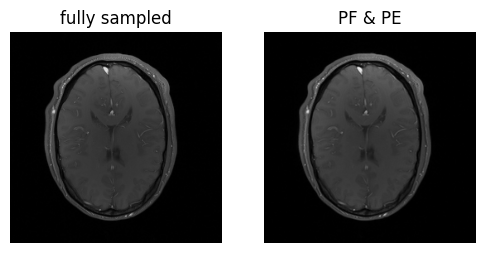
Voila! We’ve got the same brains, and they’re the same size!

More about operators

The Fourier Operator

In MRpro, we have a smart FourierOp operator, that automatically does the resorting and can handle non-cartesian data as well. For cartesian data, it internally does exactly the two steps we just did manually. The operator can be also be created from an existing KData object This is the recommended way to transform k-space data.

fourier_op = mrpro.operators.FourierOp.from_kdata(kdata_pe_pf)
# no need for and explicit CartesianSamplingOp anymore!
(img_pe_pf,) = fourier_op.adjoint(kdata_pe_pf.data)
magnitude_pe_pf = img_pe_pf.abs().square().sum(dim=-4).sqrt().squeeze()
show_images(magnitude_fully_sampled, magnitude_pe_pf, titles=['fully sampled', 'PF & PE'])

That was easy! But wait a second — something still looks a bit off. In the bottom left corner, it seems like there’s a “hole” in the brain. That definitely shouldn’t be there.

The issue is that we combined the data from the different coils using a root-sum-of-squares approach. While it’s simple, it’s not the ideal method. Typically, coil sensitivity maps are calculated to combine the data from different coils. In MRpro, you can do this by calculating coil sensitivity data and then creating a SensitivityOp to combine the data after image reconstruction.

Sensitivity Operator

We have different options for calculating coil sensitivity maps from the image data of the various coils. Here, we’re going to use the Walsh method.

# Calculate coil sensitivity maps
(img_pe_pf,) = fft_op.adjoint(*cart_sampling_op.adjoint(kdata_pe_pf.data))

# This algorithms is designed to calculate coil sensitivity maps for each other dimension.
csm_data = mrpro.algorithms.csm.walsh(img_pe_pf[0, ...], smoothing_width=5)[None, ...]

# Create SensitivityOp
csm_op = mrpro.operators.SensitivityOp(csm_data)

# Reconstruct coil-combined image
(img_walsh_combined,) = csm_op.adjoint(*fourier_op.adjoint(kdata_pe_pf.data))
magnitude_walsh_combined = img_walsh_combined.abs().squeeze()
show_images(magnitude_pe_pf, magnitude_walsh_combined, titles=['RSS', 'Adaptive Combination'])

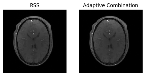
Tada! The “hole” is gone, and the image looks much better 🎉.

When we reconstructed the image, we called the adjoint method of several different operators one after the other. That was a bit cumbersome. To make our life easier, MRpro allows to combine the operators first, get the adjoint of the composite operator and then later call this adjoint composite operator.

### Operator Composition
# Create composite operator
adjoint_operator = (fourier_op @ csm_op).H
(magnitude_pe_pf,) = adjoint_operator(kdata_pe_pf.data)
magnitude_pe_pf = magnitude_pe_pf.abs().squeeze()
show_images(magnitude_pe_pf, titles=['PF & PE'])

Although we now have got a nice looking image, it was still a bit cumbersome to create it. We had to define several different operators and chain them together. Wouldn’t it be nice if this could be done automatically?

That is why we also included some top-level reconstruction algorithms in MRpro. For this whole steps from above, we can simply use a DirectReconstruction. Reconstruction algorithms can be instantiated from only the information in the KData object.

In contrast to operators, top-level reconstruction algorithms operate on the data objects of MRpro, i.e. the input is a KData object and the output is an IData object containing the reconstructed image data. To get its magnitude, we can call the rss method.

# Create DirectReconstruction object from KData object
direct_recon_pe_pf = mrpro.algorithms.reconstruction.DirectReconstruction(kdata_pe_pf)

# Reconstruct image by calling the DirectReconstruction object
idat_pe_pf = direct_recon_pe_pf(kdata_pe_pf)

This is much simpler — everything happens in the background, so we don’t have to worry about it.

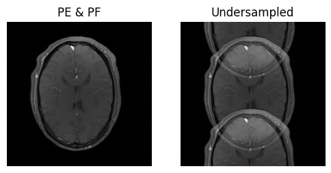
Reconstruction of undersampled data

Let’s finally try it on the undersampled dataset.

kdata_us = mrpro.data.KData.from_file(
    data_folder / 'cart_t1_msense_integrated.mrd',
    mrpro.data.traj_calculators.KTrajectoryCartesian(),
)
direct_recon_us = mrpro.algorithms.reconstruction.DirectReconstruction(kdata_us)
idat_us = direct_recon_us(kdata_us)

show_images(idat_pe_pf.rss().squeeze(), idat_us.rss().squeeze(), titles=['PE & PF', 'Undersampled'])

Using Calibration Data

We used the same data for coil sensitivity calculation as for image reconstruction (auto-calibration). Another approach is to acquire a few calibration lines in the center of k-space to create a low-resolution, fully sampled image. In our example data from Siemens scanners, these lines are part of the dataset. As they aren’t meant to be used for image reconstruction, only for calibration, i.e., coil sensitivity calculation, and are labeled in the data as such, they are ignored by the default acquisition_filter_criterion of from_file. However, we can change the filter criterion to is_coil_calibration_acquisition to read in only these acquisitions.

Note

There are already some other filter criteria available, see mrpro.data.acq_filters. You can also implement your own function returning whether to include an acquisition

kdata_calib_lines = mrpro.data.KData.from_file(
    data_folder / 'cart_t1_msense_integrated.mrd',
    mrpro.data.traj_calculators.KTrajectoryCartesian(),
    acquisition_filter_criterion=mrpro.data.acq_filters.is_coil_calibration_acquisition,
)

direct_recon_calib_lines = mrpro.algorithms.reconstruction.DirectReconstruction(kdata_calib_lines)
idat_calib_lines = direct_recon_calib_lines(kdata_calib_lines)

If we look at the reconstructed image, we see it is low resolution..

show_images(idat_calib_lines.rss().squeeze(), titles=['Calibration Image'])

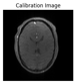
..but it is good enough to calculate coil sensitivity maps:

# The coil sensitivity maps
assert direct_recon_calib_lines.csm is not None
show_images(
    *direct_recon_calib_lines.csm.data[0].abs().squeeze(),
    titles=[f'|CSM {i}|' for i in range(direct_recon_calib_lines.csm.data.size(-4))],
)

Reconstruction

We can now use these CSMs in a new DirectReconstruction:

direct_recon_us_csm = mrpro.algorithms.reconstruction.DirectReconstruction(kdata_us, csm=direct_recon_calib_lines.csm)
idat_us_csm = direct_recon_us_csm(kdata_us)
show_images(idat_us.rss().squeeze(), idat_us_csm.rss().squeeze(), titles=['Autocalibration', 'Calibration Lines'])

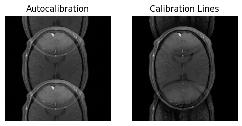
As expected, we still see undersampling artifacts in the image. In order to get rid of them, we try can a more sophisticated reconstruction method, such as the iterative SENSE algorithm. As you might have guessed, these are also included in MRpro: Instead of the DirectReconstruction, we can use IterativeSENSEReconstruction:

sense_recon_us = mrpro.algorithms.reconstruction.IterativeSENSEReconstruction(
    kdata_us,
    csm=direct_recon_calib_lines.csm,
    n_iterations=8,
)
idat_us_sense = sense_recon_us(kdata_us)
show_images(idat_us_sense.rss().squeeze(), titles=['Iterative SENSE'])

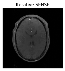
This looks better! More information about the iterative SENSE reconstruction and its implementation in MRpro can be found in the examples Iterative SENSE reconstruction of 2D golden angle radial data and Regularized iterative SENSE reconstruction of 2D golden angle radial data.