T2 Mapping - T2prep FLASH#
T2 mapping using a Cartesian FLASH sequence with T2-preparation pulses with different T2-preparation times.
Imports#
import tempfile
from pathlib import Path

import matplotlib.pyplot as plt
import MRzeroCore as mr0
import numpy as np
import torch
from cmap import Colormap
from einops import rearrange
from mrpro.algorithms.reconstruction import DirectReconstruction
from mrpro.data import KData
from mrpro.data import SpatialDimension
from mrpro.data.traj_calculators import KTrajectoryCartesian
from mrpro.operators import DictionaryMatchOp
from mrpro.operators.models import MonoExponentialDecay

from mrseq.scripts.t2_t2prep_flash import main as create_seq
from mrseq.utils import sys_defaults
/opt/hostedtoolcache/Python/3.12.13/x64/lib/python3.12/site-packages/tqdm/auto.py:21: TqdmWarning: IProgress not found. Please update jupyter and ipywidgets. See https://ipywidgets.readthedocs.io/en/stable/user_install.html
  from .autonotebook import tqdm as notebook_tqdm
Settings#
We are going to use a numerical phantom with a matrix size of 128 x 128.
image_matrix_size = [128, 128]
t2_prep_echo_times = np.array([0.0, 0.02, 0.08])

tmp = tempfile.TemporaryDirectory()
fname_mrd = Path(tmp.name) / 't2.mrd'
Create the digital phantom#
We use the standard Brainweb phantom from MRzero, but we set the B0-field and B1-field to be constant everywhere. This sequence is designed for cardiac applications and so we restrict the T1 and T2 values to reasonable values expected in the heart.
phantom = mr0.util.load_phantom(image_matrix_size)
phantom.T1[phantom.T1 > 2] = 2
phantom.T2[phantom.T2 > 0.1] = 0.1
phantom.B0[:] = 0
phantom.B1[:] = 1
Create the T2prep FLASH sequence#
To create the FLASH sequence with different T2-preparation pulses, we use the previously imported t2_t2_prep_flash script.
For in-vivo applications we have to make sure the sequence can be run within a breathhold. This would require undersampling (acceleration > 1) and obtaining a high number of phase encoding points in each cardiac cycle. This will impair the accuracy of the obtained T2 maps. For the evaluation here we can make the sequence longer to increase accuracy.
sequence, fname_seq = create_seq(
    system=sys_defaults,
    t2_prep_echo_times=t2_prep_echo_times,
    fov_xy=float(phantom.size.numpy()[0]),
    n_readout=image_matrix_size[0],
    acceleration=1,
    n_pe_points_per_cardiac_cycle=8,
    show_plots=False,
    test_report=False,
    timing_check=False,
)
Current echo time = 2.263 ms
Current repetition time = 4.540 ms
Acquisition window per cardiac cycle = 36.320 ms

Saving sequence file 't2_t2prep_flash_200fov_128nx_1us_.seq' into folder '/home/runner/work/mrseq/mrseq/examples/output'.
Simulate the sequence#
Now, we pass the sequence and the phantom to the MRzero simulation and save the simulated signal as an (ISMR)MRD file.
mr0_sequence = mr0.Sequence.import_file(str(fname_seq.with_suffix('.seq')))
signal, ktraj_adc = mr0.util.simulate(mr0_sequence, phantom, accuracy=1e-1)
mr0.sig_to_mrd(fname_mrd, signal, sequence)
>>>> Rust - compute_graph(...) >>>
Converting Python -> Rust: 0.006035387 s
Compute Graph
Computing Graph: 0.36415592 s
Analyze Graph
Analyzing Graph: 0.005791748 s
Converting Rust -> Python: 0.057797205 s
<<<< Rust <<<<
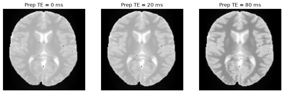
Reconstruct the images with different T2-preparation pulses.#
We use MRpro for the image reconstruction.
kdata = KData.from_file(fname_mrd, trajectory=KTrajectoryCartesian())
kdata.header.encoding_matrix = SpatialDimension(z=1, y=image_matrix_size[1], x=image_matrix_size[0] * 2)
kdata.header.recon_matrix = SpatialDimension(z=1, y=image_matrix_size[1], x=image_matrix_size[0])
recon = DirectReconstruction(kdata, csm=None)
idata = recon(kdata)
/opt/hostedtoolcache/Python/3.12.13/x64/lib/python3.12/site-packages/mrpro/data/KData.py:166: UserWarning: No vendor information found. Assuming Siemens time stamp format.
  warnings.warn('No vendor information found. Assuming Siemens time stamp format.', stacklevel=1)
We can now plot the images with different T2-preparation times.
idat = idata.data.abs().numpy().squeeze()
fig, ax = plt.subplots(1, idat.shape[0], figsize=(4 * idat.shape[0], 4))
for i in range(idat.shape[0]):
    ax[i].imshow(idat[i, :, :], cmap='gray')
    ax[i].set_title(f'Prep TE = {int(t2_prep_echo_times[i] * 1000)} ms')
    ax[i].set_xticks([])
    ax[i].set_yticks([])
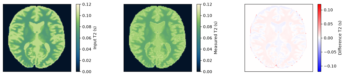
Estimate the T2 maps#
We use a dictionary matching approach to estimate the T2 maps. Afterward, we compare them to the input and ensure they match.
dictionary = DictionaryMatchOp(
    MonoExponentialDecay(decay_time=torch.tensor(t2_prep_echo_times, dtype=torch.float32)),
    index_of_scaling_parameter=0,
)
dictionary.append(torch.tensor(1.0), torch.linspace(0.001, 0.15, 1000)[None, :])
m0_match, t2_match = dictionary(idata.data[:, 0, 0])

t2_input = np.roll(rearrange(phantom.T2.numpy().squeeze()[::-1, ::-1], 'x y -> y x'), shift=(1, 1), axis=(0, 1))
obj_mask = np.zeros_like(t2_input)
obj_mask[t2_input > 0] = 1
t2_measured = t2_match.numpy().squeeze() * obj_mask

fig, ax = plt.subplots(1, 3, figsize=(15, 3))
for cax in ax:
    cax.set_xticks([])
    cax.set_yticks([])

im = ax[0].imshow(t2_input, vmin=0, vmax=0.12, cmap=Colormap('navia').to_mpl())
fig.colorbar(im, ax=ax[0], label='Input T2 (s)')

im = ax[1].imshow(t2_measured, vmin=0, vmax=0.12, cmap=Colormap('navia').to_mpl())
fig.colorbar(im, ax=ax[1], label='Measured T2 (s)')

im = ax[2].imshow(t2_measured - t2_input, vmin=-0.12, vmax=0.12, cmap='bwr')
fig.colorbar(im, ax=ax[2], label='Difference T2 (s)')

relative_error = np.sum(np.abs(t2_input - t2_measured)) / np.sum(np.abs(t2_input))
print(f'Relative error {relative_error}')
assert relative_error < 0.06
Relative error 0.0529717281460762