T1 Mapping - MOLLI#
T1 mapping using a spin echo sequence where a single readout line is acquired after an inversion pulse. Multiple images are obtained at different inversion times. A long repetition time (TR) is used to ensure full signal recovery before the next k-space line is acquired.
Imports#
import tempfile
from pathlib import Path

import matplotlib.pyplot as plt
import MRzeroCore as mr0
import numpy as np
import torch
from cmap import Colormap
from einops import rearrange
from mrpro.algorithms.reconstruction import IterativeSENSEReconstruction
from mrpro.data import CsmData
from mrpro.data import KData
from mrpro.data import SpatialDimension
from mrpro.data.acq_filters import is_coil_calibration_acquisition
from mrpro.data.traj_calculators import KTrajectoryCartesian
from mrpro.operators import DictionaryMatchOp
from mrpro.operators.models import MOLLI
from mrpro.phantoms.coils import birdcage_2d

from mrseq.scripts.t1_molli_bssfp import main as create_seq
from mrseq.utils import sys_defaults
/opt/hostedtoolcache/Python/3.12.13/x64/lib/python3.12/site-packages/tqdm/auto.py:21: TqdmWarning: IProgress not found. Please update jupyter and ipywidgets. See https://ipywidgets.readthedocs.io/en/stable/user_install.html
  from .autonotebook import tqdm as notebook_tqdm
Settings#
We are going to use a numerical phantom with a matrix size of 128 x 128. The repetition time is set to 20 seconds to ensure we can accurately estimate long T1 times of the CSF.
image_matrix_size = [64, 64]

tmp = tempfile.TemporaryDirectory()
fname_mrd = Path(tmp.name) / 't1_molli.mrd'
Create the digital phantom#
We use the standard Brainweb phantom from MRzero, but we choose the B1-field to be constant everywhere.
im_dims = SpatialDimension(z=1, y=image_matrix_size[1], x=image_matrix_size[0])
coil_maps = birdcage_2d(6, image_dimensions=im_dims, relative_radius=0.8)

phantom = mr0.util.load_phantom(image_matrix_size)
phantom.B1[:] = 1.0
phantom.coil_sens = rearrange(coil_maps[0, ...], 'coils z y x -> coils x y z')
Create the MOLLI bSSFP sequence#
To create the MOLLI bSSFP sequence, we use the previously imported t1_molli_bssfp script.
sequence, fname_seq = create_seq(
    system=sys_defaults,
    test_report=False,
    timing_check=False,
    fov_xy=float(phantom.size.numpy()[0]),
    n_readout=image_matrix_size[0],
    acceleration=2,
)
Current receiver bandwidth = 1042 Hz/pixel

Current echo time = 1.604 ms
Current repetition time = 3.220 ms
Acquisition window per cardiac cycle = 122.360 ms

Saving sequence file 't1_molli_bssfp_200fov_64nx_2us.seq' into folder '/home/runner/work/mrseq/mrseq/examples/output'.
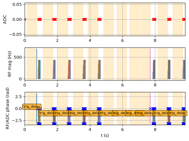
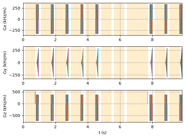
Simulate the sequence#
Now, we pass the sequence and the phantom to the MRzero simulation and save the simulated signal as an (ISMR)MRD file.
mr0_sequence = mr0.Sequence.import_file(str(fname_seq.with_suffix('.seq')))
signal, ktraj_adc = mr0.util.simulate(mr0_sequence, phantom, accuracy=1e-2)
mr0.sig_to_mrd(fname_mrd, signal, sequence)
>>>> Rust - compute_graph(...) >>>
Converting Python -> Rust: 0.00269048 s
Compute Graph
Computing Graph: 0.413667 s
Analyze Graph
Analyzing Graph: 0.01187613 s
Converting Rust -> Python: 0.12723595 s
<<<< Rust <<<<
Reconstruct the images at different inversion times#
We use MRpro for the image reconstruction.
kdata = KData.from_file(fname_mrd, trajectory=KTrajectoryCartesian())
kdata.header.encoding_matrix = SpatialDimension(z=1, y=image_matrix_size[1], x=image_matrix_size[0] * 2)
kdata.header.recon_matrix = SpatialDimension(z=1, y=image_matrix_size[1], x=image_matrix_size[0])


kdata_calib = KData.from_file(
    fname_mrd, trajectory=KTrajectoryCartesian(), acquisition_filter_criterion=is_coil_calibration_acquisition
)
kdata_calib.header.encoding_matrix = SpatialDimension(z=1, y=image_matrix_size[1], x=image_matrix_size[0] * 2)
kdata_calib.header.recon_matrix = SpatialDimension(z=1, y=image_matrix_size[1], x=image_matrix_size[0])
csm = CsmData.from_kdata_inati(kdata_calib[0], downsampled_size=64, smoothing_width=9)
recon = IterativeSENSEReconstruction(kdata, csm=csm, n_iterations=8)
idata = recon(kdata)
/opt/hostedtoolcache/Python/3.12.13/x64/lib/python3.12/site-packages/mrpro/data/KData.py:166: UserWarning: No vendor information found. Assuming Siemens time stamp format.
  warnings.warn('No vendor information found. Assuming Siemens time stamp format.', stacklevel=1)
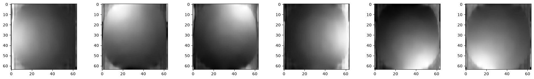
We visualize the coil sensitivity maps which we used for the iterative SENSE reconstruction.
fig, ax = plt.subplots(1, csm.shape[1], figsize=(3 * idata.shape[0], 3))
for i in range(csm.shape[1]):
    ax[i].imshow(csm.data[0, i, 0, :, :].abs(), cmap='gray')
/opt/hostedtoolcache/Python/3.12.13/x64/lib/python3.12/site-packages/matplotlib/cbook.py:713: DeprecationWarning: __array__ implementation doesn't accept a copy keyword, so passing copy=False failed. __array__ must implement 'dtype' and 'copy' keyword arguments. To learn more, see the migration guide https://numpy.org/devdocs/numpy_2_0_migration_guide.html#adapting-to-changes-in-the-copy-keyword
  x = np.array(x, subok=True, copy=copy)
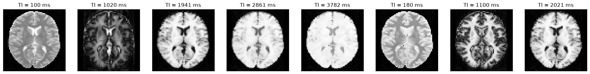
We can now plot the images at different inversion times.
idat = idata.rss().abs().numpy().squeeze()
acquisition_time_stamp = idata.header.acquisition_time_stamp.squeeze()
ti = np.concatenate(
    (
        idata.header.ti[0] + acquisition_time_stamp[:5] - acquisition_time_stamp[0],
        idata.header.ti[1] + acquisition_time_stamp[5:] - acquisition_time_stamp[5],
    )
)
fig, ax = plt.subplots(1, idat.shape[0], figsize=(3 * idata.shape[0], 3))
for i in range(idat.shape[0]):
    ax[i].imshow(idat[i, :, :], cmap='gray')
    ax[i].set_title(f'TI = {int(np.round(ti[i] * 1000))} ms')
    ax[i].set_xticks([])
    ax[i].set_yticks([])
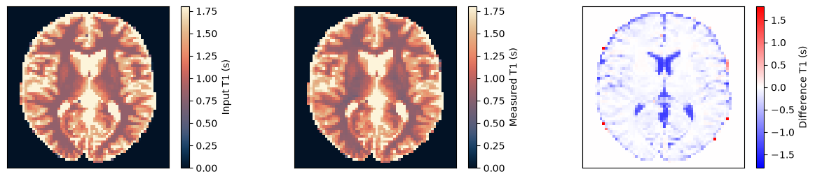
Estimate the T1 maps#
We use a dictionary matching approach to estimate the T1 maps. Afterward, we compare them to the input and ensure they match.
dictionary = DictionaryMatchOp(MOLLI(ti=torch.as_tensor(ti, dtype=torch.float32)), index_of_scaling_parameter=0)
dictionary.append(
    torch.tensor(1.0), torch.linspace(0.1, 5.0, 300)[None, :, None], torch.linspace(0.1, 5.0, 300)[None, None, :]
)
m0_match, c_match, t1_match = dictionary(idata.data)

t1_input = np.roll(rearrange(phantom.T1.numpy().squeeze()[::-1, ::-1], 'x y -> y x'), shift=(1, 1), axis=(0, 1))
obj_mask = np.zeros_like(t1_input)
obj_mask[t1_input > 0] = 1
t1_measured = t1_match.numpy().squeeze() * obj_mask

fig, ax = plt.subplots(1, 3, figsize=(15, 3))
for cax in ax:
    cax.set_xticks([])
    cax.set_yticks([])

im = ax[0].imshow(t1_input, vmin=0, vmax=1.8, cmap=Colormap('lipari').to_mpl())
fig.colorbar(im, ax=ax[0], label='Input T1 (s)')

im = ax[1].imshow(t1_measured, vmin=0, vmax=1.8, cmap=Colormap('lipari').to_mpl())
fig.colorbar(im, ax=ax[1], label='Measured T1 (s)')

im = ax[2].imshow(t1_measured - t1_input, vmin=-1.8, vmax=1.8, cmap='bwr')
fig.colorbar(im, ax=ax[2], label='Difference T1 (s)')

relative_error = np.sum(np.abs(t1_input - t1_measured)) / np.sum(np.abs(t1_input))
print(f'Relative error {relative_error}')
assert relative_error < 0.12
Relative error 0.1162678524851799