T1 and T2 Mapping - Spiral cMRF

T1 and T2 mapping with a cardiac MR Fingerprinting sequence using a spiral readout.

Imports

import tempfile
from pathlib import Path

import matplotlib.pyplot as plt
import MRzeroCore as mr0
import numpy as np
import torch
from cmap import Colormap
from einops import rearrange
from mrpro.algorithms.reconstruction import DirectReconstruction
from mrpro.data import CsmData
from mrpro.data import KData
from mrpro.data.traj_calculators import KTrajectoryIsmrmrd
from mrpro.operators import AveragingOp
from mrpro.operators import DictionaryMatchOp
from mrpro.operators.models import CardiacFingerprinting

from mrseq.scripts.t1_t2_spiral_cmrf import main as create_seq
from mrseq.utils import combine_ismrmrd_files
from mrseq.utils import sys_defaults

Settings

A MRF sequence relies on complex signal dynamics during the data acquisition. This is computationally demanding to simulate. To keep run times short, we are therefore going to use only a very low-resolution numerical phantom with a matrix size of 48 x 48.

image_matrix_size = [48, 48]
t2_prep_echo_times = (0.03, 0.05, 0.08)

tmp = tempfile.TemporaryDirectory()
fname_mrd = Path(tmp.name) / 'cmrf.mrd'

Create the digital phantom

We use the standard Brainweb phantom from MRzero, but we set the B1-field to be constant everywhere. This sequence is also optimized for T1 and T2 mapping of the myocardium and not for the long T1 and T2 times of the CSF. We are therefore going to limit the highest T1 values to 2s and the highest T2 values to 0.2s.

phantom = mr0.util.load_phantom(image_matrix_size)
phantom.B1[:] = 1.0
phantom.T1[phantom.T1 > 2] = 2
phantom.T2[phantom.T2 > 0.2] = 0.2

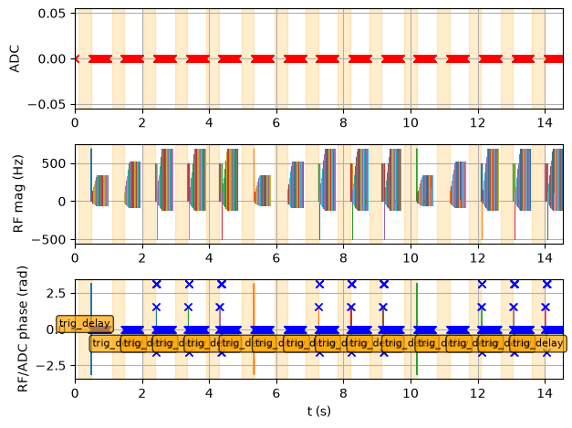
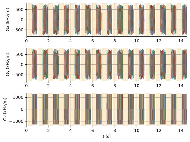
Create the spiral cardiac MRF sequence

To create the cMRF sequence, we use the previously imported t1_t2_spiral_cmrf.

sequence, fname_seq = create_seq(
    system=sys_defaults,
    test_report=False,
    timing_check=False,
    fov_xy=float(phantom.size.numpy()[0]),
    n_readout=image_matrix_size[0],
    t2_prep_echo_times=t2_prep_echo_times,
    spiral_undersampling=1,
)

Target undersampling: 1 -  achieved undersampling: 1.00 FOV: 0.200 (k-sapce center) - 0.181 (k-space edge)
Receiver bandwidth: 2083 Hz/pixel

 Manual timing calculations:

 shortest possible TR = 3.310 ms

 final TR = 10.000 ms

Saving sequence file 't1_t2_spiral_cmrf_200fov_48px_variable_trig_delay.seq' into folder '/home/runner/work/mrseq/mrseq/examples/output'.

Simulate the sequence

Now, we pass the sequence and the phantom to the MRzero simulation and save the simulated signal as an (ISMR)MRD file.

mr0_sequence = mr0.Sequence.import_file(str(fname_seq.with_suffix('.seq')))
signal, ktraj_adc = mr0.util.simulate(mr0_sequence, phantom, accuracy=1e-3)
mr0.sig_to_mrd(fname_mrd, signal, sequence)
combine_ismrmrd_files(fname_mrd, Path(f'{fname_seq}_header.h5'))

>>>> Rust - compute_graph(...) >>>

Converting Python -> Rust: 0.004820329 s
Compute Graph
Computing Graph: 9.071514 s
Analyze Graph
Analyzing Graph: 0.48916358 s
Converting Rust -> Python: 3.448659 s
<<<< Rust <<<<

<ismrmrd.hdf5.Dataset at 0x7fe4245bf3b0>

Reconstruct series of images showing the dynamic contrast change

We use MRpro for the image reconstruction.

kdata = KData.from_file(str(fname_mrd).replace('.mrd', '_with_traj.mrd'), trajectory=KTrajectoryIsmrmrd())
csm = CsmData.from_kdata_inati(kdata, downsampled_size=24)

n_acq_per_image = 20
n_overlap = 10
n_acq_per_block = 47
n_blocks = 15

idx_in_block = torch.arange(n_acq_per_block).unfold(0, n_acq_per_image, n_acq_per_image - n_overlap)
split_indices = (n_acq_per_block * torch.arange(n_blocks)[:, None, None] + idx_in_block).flatten(end_dim=1)
kdata_split = kdata[..., split_indices, :]

reco = DirectReconstruction(kdata_split, csm=csm)
idata = reco(kdata_split)

/opt/hostedtoolcache/Python/3.12.12/x64/lib/python3.12/site-packages/mrpro/data/KData.py:166: UserWarning: No vendor information found. Assuming Siemens time stamp format.
  warnings.warn('No vendor information found. Assuming Siemens time stamp format.', stacklevel=1)

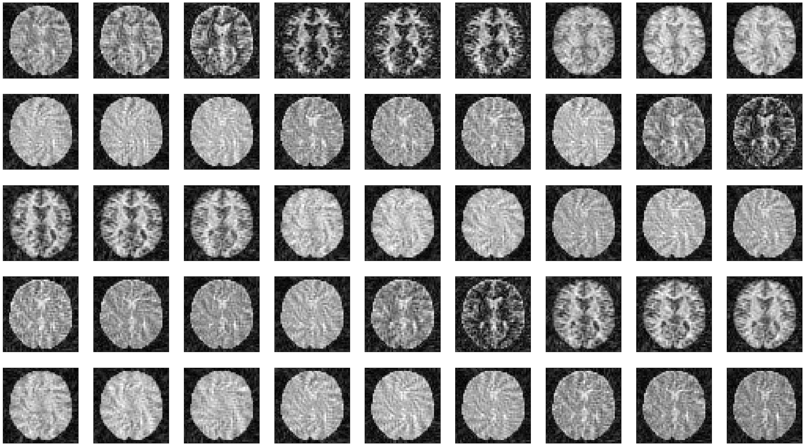
We can now plot the images at different time points along the acquisition.

idat = idata.data.abs().numpy().squeeze()
fig, ax = plt.subplots(5, idat.shape[0] // 5, figsize=(4 * idata.shape[0] // 5, 5 * 4))
ax = ax.flatten()
for i in range(idat.shape[0]):
    ax[i].imshow(idat[i, :, :], cmap='gray')
    ax[i].set_xticks([])
    ax[i].set_yticks([])

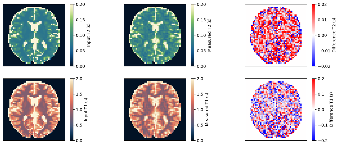
Estimate the T1 and T2 maps

We use a dictionary matching approach to estimate the T1 and T2 maps. Afterward, we compare them to the input and ensure they match.

model = AveragingOp(dim=0, idx=split_indices) @ CardiacFingerprinting(
    kdata.header.acq_info.acquisition_time_stamp.squeeze(),
    echo_time=kdata.header.te[0],
    repetition_time=kdata.header.tr[0],
    t2_prep_echo_times=t2_prep_echo_times,
)
dictionary = DictionaryMatchOp(model, index_of_scaling_parameter=0)
t1_keys = torch.arange(0.05, 3, 0.05)[:, None]
t2_keys = torch.arange(0.01, 0.3, 0.01)[None, :]
m0_keys = torch.tensor(1.0)
dictionary.append(m0_keys, t1_keys, t2_keys)
m0_match, t1_match, t2_match = dictionary(idata.data)

t1_input = np.roll(rearrange(phantom.T1.numpy().squeeze()[::-1, ::-1], 'x y -> y x'), shift=(1, 1), axis=(0, 1))
t2_input = np.roll(rearrange(phantom.T2.numpy().squeeze()[::-1, ::-1], 'x y -> y x'), shift=(1, 1), axis=(0, 1))
obj_mask = np.zeros_like(t2_input)
obj_mask[t2_input > 0] = 1
t2_measured = t2_match.numpy().squeeze() * obj_mask
t1_measured = t1_match.numpy().squeeze() * obj_mask

fig, ax = plt.subplots(2, 3, figsize=(15, 6))
for cax in ax.flatten():
    cax.set_xticks([])
    cax.set_yticks([])

im = ax[0, 0].imshow(t2_input, vmin=0, vmax=0.2, cmap=Colormap('navia').to_mpl())
fig.colorbar(im, ax=ax[0, 0], label='Input T2 (s)')

im = ax[0, 1].imshow(t2_measured, vmin=0, vmax=0.2, cmap=Colormap('navia').to_mpl())
fig.colorbar(im, ax=ax[0, 1], label='Measured T2 (s)')

im = ax[0, 2].imshow(t2_measured - t2_input, vmin=-0.02, vmax=0.02, cmap='bwr')
fig.colorbar(im, ax=ax[0, 2], label='Difference T2 (s)')

im = ax[1, 0].imshow(t1_input, vmin=0, vmax=2, cmap=Colormap('lipari').to_mpl())
fig.colorbar(im, ax=ax[1, 0], label='Input T1 (s)')

im = ax[1, 1].imshow(t1_measured, vmin=0, vmax=2, cmap=Colormap('lipari').to_mpl())
fig.colorbar(im, ax=ax[1, 1], label='Measured T1 (s)')

im = ax[1, 2].imshow(t1_measured - t1_input, vmin=-0.2, vmax=0.2, cmap='bwr')
fig.colorbar(im, ax=ax[1, 2], label='Difference T1 (s)')

relative_error_t2 = np.sum(np.abs(t2_input - t2_measured)) / np.sum(np.abs(t2_input))
relative_error_t1 = np.sum(np.abs(t1_input - t1_measured)) / np.sum(np.abs(t1_input))
print(f'Relative error for T2: {relative_error_t2} and for T1: {relative_error_t1}')
assert relative_error_t2 < 0.15
assert relative_error_t1 < 0.08

Relative error for T2: 0.13122183084487915 and for T1: 0.07772935181856155