GRPE FLASH Dixon

Golden radial phase encoding acquisition with a 3-point Dixon gradient echo readout. More detailed information on the acquisition can be found here:

Mayer et al 2022. Cardio‐respiratory motion‐corrected 3D cardiac water‐fat MRI using model‐based image reconstruction. MRM. https://doi.org/10.1002/mrm.29284

Imports

import tempfile
import time
from pathlib import Path
from urllib.request import urlretrieve

import matplotlib.pyplot as plt
import MRzeroCore as mr0
import numpy as np
import scipy as sp
import torch
from einops import rearrange
from mrpro.algorithms.reconstruction import DirectReconstruction
from mrpro.data import KData
from mrpro.data.enums import AcqFlags
from mrpro.data.traj_calculators import KTrajectoryIsmrmrd
from mrpro.operators.models import SpoiledGRE
from scipy.interpolate import interp1d

from mrseq.scripts.grpe_flash_dixon import main as create_seq
from mrseq.utils import combine_ismrmrd_files
from mrseq.utils import sys_defaults

Settings

We are going to use a small numerical phantom with a matrix size of 32 x 32 x 32 to reduce run times. To ensure we really acquire all data in the steady state, we use a large number of dummy excitations before the actual image acquisition.

# Acquisition parameters
flip_angle_degree = 12
n_dummy_spokes = 10
image_matrix_size = [32, 32, 32]  # x,y,z

# Output path
tmp = tempfile.TemporaryDirectory()
fname_mrd = Path(tmp.name) / 'grpe_flash_dixon.mrd'

Digital Phantom

We use the Brainweb phantom from MRzero, interpolated to our desired matrix size, with uniform B1 field.

# Load 3D brainweb phantom
urlretrieve(
    'https://github.com/MRsources/MRzero-Core/raw/main/documentation/playground_mr0/subject05.npz', 'subject05.npz'
)

obj_p = mr0.VoxelGridPhantom.brainweb('subject05.npz')
phantom = obj_p.interpolate(*image_matrix_size)
phantom.size[2] = phantom.size[1]  # GRPE assumes isotropic voxels in y-z plane
phantom.B1[:] = 1.0

/opt/hostedtoolcache/Python/3.12.13/x64/lib/python3.12/site-packages/MRzeroCore/phantom/voxel_grid_phantom.py:192: DeprecationWarning: brainweb() will be removed in a future version, use load() instead
  warn("brainweb() will be removed in a future version, use load() instead", DeprecationWarning)

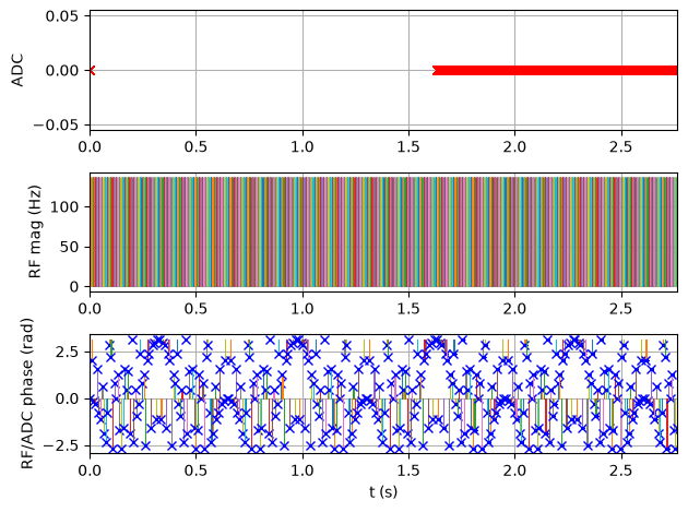
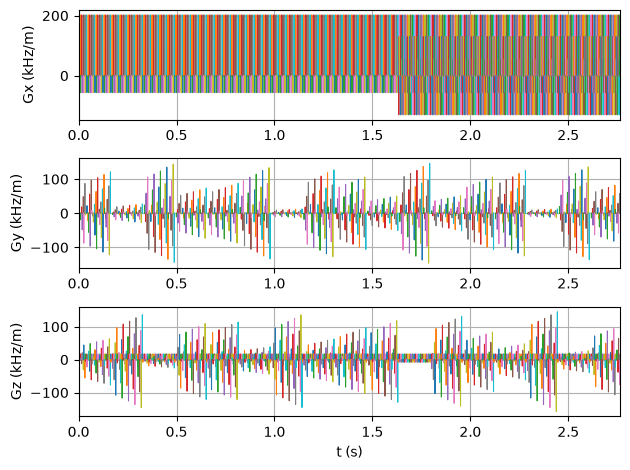
Create the 3D GRPE FLASH Sequence

Generate a golden radial phase encoding FLASH sequence with partial Fourier along the RPE lines and partial echo along the readout.

sequence, fname_seq = create_seq(
    system=sys_defaults,
    test_report=False,
    timing_check=False,
    rf_flip_angle=flip_angle_degree,
    fov_x=float(phantom.size.numpy()[0]),
    fov_y=float(phantom.size.numpy()[1]),
    fov_z=float(phantom.size.numpy()[1]),
    n_readout=32,
    n_rpe_points=32,
    n_rpe_points_per_shot=4,
    n_rpe_spokes=48,
    partial_echo_factor=0.7,
    partial_fourier_factor=0.7,
    n_dummy_spokes=n_dummy_spokes,
)

Number of phase encoding points 20 with partial Fourier factor 0.7

Current echo time = 1.310 ms
Current repetition time = 8.130 ms

Saving sequence file 'grpe_flash_dixon_fov192_192_192mm_32_32_48_3ne.seq' into folder '/home/runner/work/mrseq/mrseq/examples/output'.

Simulate the Sequence

Pass the sequence and phantom to the MRzero simulation engine and save the signal as an ISMRMRD file.

mr0_sequence = mr0.Sequence.import_file(str(fname_seq.with_suffix('.seq')))
tstart = time.time()
signal, ktraj_adc = mr0.util.simulate(mr0_sequence, phantom, accuracy=1e0)
print(f'Simulation time: {(time.time() - tstart) / 60:.2f} min')
mr0.sig_to_mrd(fname_mrd, signal, sequence)
combine_ismrmrd_files(fname_mrd, Path(f'{fname_seq}_header.h5'))

>>>> Rust - compute_graph(...) >>>
Converting Python -> Rust: 0.00723438 s
Compute Graph
Computing Graph: 26.779974 s
Analyze Graph
Analyzing Graph: 1.1849208 s
Converting Rust -> Python: 9.976366 s
<<<< Rust <<<<

Simulation time: 1.61 min

<ismrmrd.hdf5.Dataset at 0x7fe2cd891820>

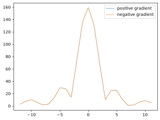
Gradient correction

We are using a bipolar readout gradient to achieve short echo times and efficient sampling. Due to hardware limitations, the positive and negative gradient lobes are not exactly the same. This can lead to small shifts of the k-space trajectory between positive and negative readout gradients. If these are not corrected for, there are linear phase errors in image space along the readout direction, which can strongly impair the fat-water separation.

There are several approaches that estimate this phase error from the imaging data. For this sequence, we acquire additional data without phase encoding, where we change the polarity of the readout gradient. First, we acquire with positive - negative - positive readout gradients and then negative - positive - negative readout gradients. We can then use a cross-correlation between the pairs of positive and negative readout gradients at the same echo times to estimate this shift and correct for it.

As a first step, we get the additional data that is labeled as ACQ_IS_PHASECORR_DATA.

kdata_corr = KData.from_file(
    str(fname_mrd).replace('.mrd', '_with_traj.mrd'),
    trajectory=KTrajectoryIsmrmrd(),
    acquisition_filter_criterion=lambda acquisition: AcqFlags.ACQ_IS_PHASECORR_DATA.value & acquisition.flags,
)

/opt/hostedtoolcache/Python/3.12.13/x64/lib/python3.12/site-packages/mrpro/data/KData.py:165: UserWarning: No vendor information found. Assuming Siemens time stamp format.
  warnings.warn('No vendor information found. Assuming Siemens time stamp format.', stacklevel=1)

To distinguish between the “positive - negative - positive” and “negative - positive - negative” acquisition, the first are labeled with the acquisition index repetition = 0 and the second with repetition = 1. We also use multiple averages to reduce noise. So let’s split it up into the different components.

sort_indices = np.lexsort(
    (
        kdata_corr.header.acq_info.idx.contrast.squeeze(),
        kdata_corr.header.acq_info.idx.repetition.squeeze(),
        kdata_corr.header.acq_info.idx.average.squeeze(),
    )
)
kdata_corr = kdata_corr[sort_indices.tolist(), ...].rearrange(
    '(average repetition contrast)... -> average repetition contrast ...',
    average=kdata_corr.header.acq_info.idx.average.unique().numel(),
    repetition=kdata_corr.header.acq_info.idx.repetition.unique().numel(),
    contrast=kdata_corr.header.acq_info.idx.contrast.unique().numel(),
)

We are going to use the first echo for the estimation of the shift. The code below will also work for the other echoes and should lead to the same shift.

echo = 0

# Get data for the current echo and compute mean over averages
kdata = torch.abs(torch.mean(kdata_corr.data[:, :, echo], dim=0)).squeeze().clone()
ktraj = kdata_corr.traj.kx[0, :, echo].squeeze().clone()

if echo % 2 == 1:  # switch positive and negative lobe to get the correct sign for the shift
    kdata = kdata[(1, 0), ...]
    ktraj = ktraj[(1, 0), ...]

kspace_start = int(ktraj[0, :].min().abs().item())
ktraj_interpolated = np.linspace(-kspace_start, kspace_start - 1, 20 * kspace_start)
kdata_interp = [
    interp1d(pos.numpy(), signal.numpy(), kind='linear', fill_value='extrapolate')(ktraj_interpolated)
    for pos, signal in zip(ktraj, kdata, strict=True)
]

plt.figure()
plt.plot(ktraj_interpolated, kdata_interp[0], label='positive gradient')
plt.plot(ktraj_interpolated, kdata_interp[1], label='negative gradient')
plt.legend()

cross_correlation = sp.signal.correlate(kdata_interp[0], kdata_interp[1], mode='same')
kspace_shift = (np.argmax(cross_correlation) - len(kdata_interp[0]) // 2) / 10  # divide by interpolation factor
print(f'K-space shift (in k-space samples): {kspace_shift}')
assert kspace_shift == 0

K-space shift (in k-space samples): 0.0

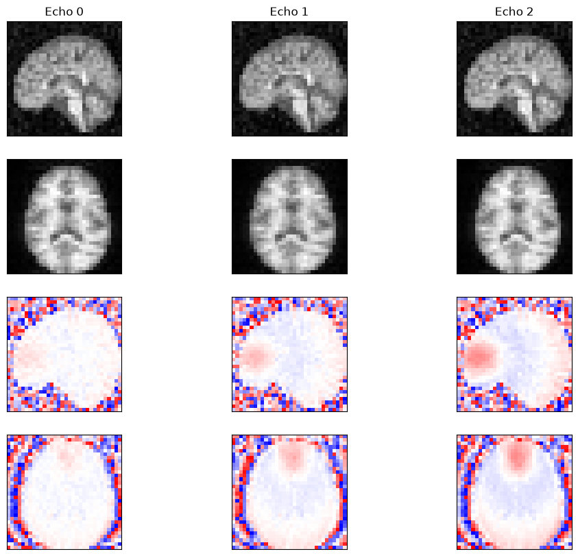
Reconstruction

Reconstruct the 3D image from the k-space data using direct reconstruction.

# Load k-space data and reconstruct
kdata = KData.from_file(
    str(fname_mrd).replace('.mrd', '_with_traj.mrd'),
    trajectory=KTrajectoryIsmrmrd(),
)

kdata.traj.kx[1] += kspace_shift  # delta_k (set to actual value if needed)

recon = DirectReconstruction(kdata, csm=None)
idata = recon(kdata)

fig, ax = plt.subplots(4, 3, figsize=(12, 10))
for cax in ax.flatten():
    cax.set_xticks([])
    cax.set_yticks([])

idat = idata.data.numpy().squeeze()
z_mid, x_mid = idat.shape[-3] // 2, idat.shape[-1] // 2

for echo in range(idat.shape[0]):
    ax[0, echo].imshow(np.abs(idat[echo, :, :, x_mid]), cmap='gray')
    ax[1, echo].imshow(np.abs(idat[echo, z_mid, :, :]), cmap='gray')
    ax[2, echo].imshow(np.angle(idat[echo, :, :, x_mid]), cmap='bwr', vmin=-np.pi, vmax=np.pi)
    ax[3, echo].imshow(np.angle(idat[echo, z_mid, :, :]), cmap='bwr', vmin=-np.pi, vmax=np.pi)
    ax[0, echo].set_title(f'Echo {echo}')

Compare to Theoretical Model

Compare the reconstructed images to a theoretical spoiled GRE signal model. We calculate \(T2^*\) using \(1/T2^* = 1/T2 + 1/T2'\).

# Calculate T2* and generate theoretical model
t2star = 1 / (1 / phantom.T2 + 1 / phantom.T2dash)

model = SpoiledGRE(
    flip_angle=np.deg2rad(flip_angle_degree),
    echo_time=kdata.header.te,
    repetition_time=kdata.header.tr,
)
idat_model = model(m0=phantom.PD, t1=phantom.T1, t2star=t2star)[0]
idat_model = idat_model.detach().abs().numpy().squeeze()
idat_model /= idat_model.max()
idat_model = np.roll(
    rearrange(idat_model[:, ::-1, ::-1, ::-1], 'echo x y z -> echo z y x'),
    shift=(1, 1, 1),
    axis=(-1, -2, -3),
)

# Create object mask
obj_mask = np.zeros_like(idat_model)
obj_mask[idat_model > 0.01] = 1

# Normalize reconstructed image
idat = idata.data.abs().squeeze().numpy()
idat = idat * obj_mask
idat /= np.percentile(idat, 99.9)

idat_diff = idat - idat_model

# Comparison: axial view (middle z-slice)
fig, ax = plt.subplots(3, 3, figsize=(12, 10))
x_mid = idat.shape[-1] // 2

for echo in range(3):
    im = ax[0, echo].imshow(idat[echo, :, :, x_mid], cmap='grey', vmin=0, vmax=1)
    ax[0, echo].set_title(f'Echo {echo} - Reconstructed')
    ax[0, echo].set_xticks([])
    ax[0, echo].set_yticks([])
    fig.colorbar(im, ax=ax[0, echo])

    im = ax[1, echo].imshow(idat_model[echo, :, :, x_mid], cmap='grey', vmin=0, vmax=1)
    ax[1, echo].set_title(f'Echo {echo} - Model')
    ax[1, echo].set_xticks([])
    ax[1, echo].set_yticks([])
    fig.colorbar(im, ax=ax[1, echo])

    im = ax[2, echo].imshow(idat_diff[echo, :, :, x_mid], cmap='bwr', vmin=-0.2, vmax=0.2)
    ax[2, echo].set_title(f'Echo {echo} - Difference')
    ax[2, echo].set_xticks([])
    ax[2, echo].set_yticks([])
    fig.colorbar(im, ax=ax[2, echo])

plt.tight_layout()
plt.show()


relative_error = np.sum(np.abs(idat_diff)) / np.sum(np.abs(idat_model))
print(f'Relative error: {relative_error:.4f}')
assert relative_error < 0.09

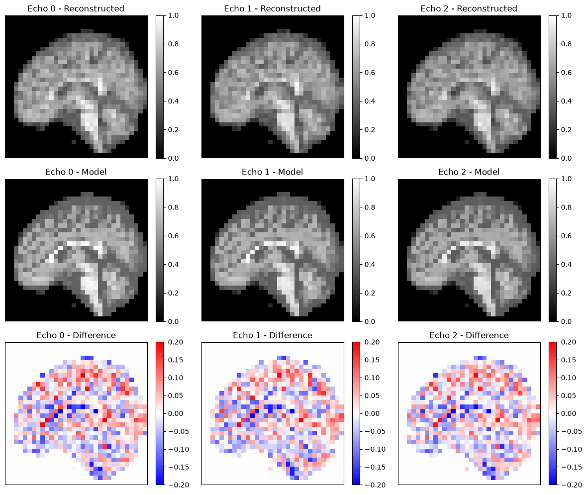
Relative error: 0.0890