# Parameters
secretsPath = "/home/runner/work/_temp/secrets.json"
QMRI Challenge ISMRM 2024 - \(T_1\) mapping
# Imports
import shutil
import tempfile
import zipfile
from pathlib import Path

import matplotlib.pyplot as plt
import torch
import zenodo_get
from einops import rearrange
from mpl_toolkits.axes_grid1 import make_axes_locatable  # type: ignore [import-untyped]
from mrpro.algorithms.optimizers import adam
from mrpro.data import IData
from mrpro.operators import MagnitudeOp
from mrpro.operators.functionals import MSE
from mrpro.operators.models import InversionRecovery
Overview
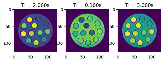
The dataset consists of images obtained at 10 different inversion times using a turbo spin echo sequence. Each inversion time is saved in a separate DICOM file. In order to obtain a \(T_1\) map, we are going to:
download the data from Zenodo
read in the DICOM files (one for each inversion time) and combine them in an IData object
define a signal model and data loss (mean-squared error) function
find good starting values for each pixel
carry out a fit using ADAM from PyTorch
Get data from Zenodo
data_folder = Path(tempfile.mkdtemp())
dataset = '10868350'
zenodo_get.zenodo_get([dataset, '-r', 5, '-o', data_folder])  # r: retries
with zipfile.ZipFile(data_folder / Path('T1 IR.zip'), 'r') as zip_ref:
    zip_ref.extractall(data_folder)
Title: Quantitative Study Group: T_1
Keywords:
Publication date: 2024-03-25
DOI: 10.5281/zenodo.10868350
Total size: 412.6 kB

Link: https://zenodo.org/records/10868350/files/T1 IR.zip   size: 412.6 kB
Checksum is correct. (ccd5f719680c4b5396ec5fb0932f66e1)
All files have been downloaded.
Create image data (IData) object with different inversion times
ti_dicom_files = data_folder.glob('**/*.dcm')
idata_multi_ti = IData.from_dicom_files(ti_dicom_files)

if idata_multi_ti.header.ti is None:
    raise ValueError('Inversion times need to be defined in the DICOM files.')
# Let's have a look at some of the images
fig, axes = plt.subplots(1, 3, squeeze=False)
for idx, ax in enumerate(axes.flatten()):
    ax.imshow(torch.abs(idata_multi_ti.data[idx, 0, 0, :, :]))
    ax.set_title(f'TI = {idata_multi_ti.header.ti[idx]:.3f}s')

Signal model and loss function
We use the model \(q\)
\(q(TI) = M_0 (1 - e^{-TI/T_1})\)
with the equilibrium magnetization \(M_0\), the inversion time \(TI\), and \(T_1\). We have to keep in mind that the DICOM images only contain the magnitude of the signal. Therefore, we need \(|q(TI)|\):
model = MagnitudeOp() @ InversionRecovery(ti=idata_multi_ti.header.ti)
As a loss function for the optimizer, we calculate the mean-squared error between the image data \(x\) and our signal model \(q\).
mse = MSE(idata_multi_ti.data.abs())
Now we can simply combine the two into a functional to solve
\( \min_{M_0, T_1} || |q(M_0, T_1, TI)| - x||_2^2\)
functional = mse @ model
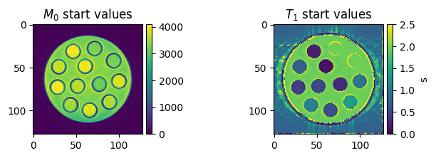
Starting values for the fit
We are trying to minimize a non-linear function \(q\). There is no guarantee that we reach the global minimum, but we can end up in a local minimum.
To increase our chances of reaching the global minimum, we can ensure that our starting values are already close to the global minimum. We need a good starting point for each pixel.
One option to get a good starting point is to calculate the signal curves for a range of \(T_1\) values and then check for each pixel which of these signal curves fits best. This is similar to what is done for MR Fingerprinting. So we are going to:
define a list of realistic \(T_1\) values (we call this a dictionary of \(T_1\) values)
calculate the signal curves corresponding to each of these \(T_1\) values
compare the signal curves to the signals of each voxel (we use the maximum of the dot-product as a metric of how well the signals fit to each other)
# Define 100 T1 values between 0.1 and 3.0 s
t1_dictionary = torch.linspace(0.1, 3.0, 100)

# Calculate the signal corresponding to each of these T1 values. We set M0 to 1, but this is arbitrary because M0 is
# just a scaling factor and we are going to normalize the signal curves.
(signal_dictionary,) = model(torch.ones(1), t1_dictionary)
signal_dictionary = signal_dictionary.to(dtype=torch.complex64)
vector_norm = torch.linalg.vector_norm(signal_dictionary, dim=0)
signal_dictionary /= vector_norm

# Calculate the dot-product and select for each voxel the T1 values that correspond to the maximum of the dot-product
n_y, n_x = idata_multi_ti.data.shape[-2:]
dot_product = torch.mm(rearrange(idata_multi_ti.data, 'other 1 z y x->(z y x) other'), signal_dictionary)
idx_best_match = torch.argmax(torch.abs(dot_product), dim=1)
t1_start = rearrange(t1_dictionary[idx_best_match], '(y x)->1 1 y x', y=n_y, x=n_x)
# The maximum absolute value observed is a good approximation for m0
m0_start = torch.amax(torch.abs(idata_multi_ti.data), 0)
# Visualize the starting values
fig, axes = plt.subplots(1, 2, figsize=(8, 2), squeeze=False)
colorbar_ax = [make_axes_locatable(ax).append_axes('right', size='5%', pad=0.05) for ax in axes[0, :]]
im = axes[0, 0].imshow(m0_start[0, 0, ...])
axes[0, 0].set_title('$M_0$ start values')
fig.colorbar(im, cax=colorbar_ax[0])
im = axes[0, 1].imshow(t1_start[0, 0, ...], vmin=0, vmax=2.5)
axes[0, 1].set_title('$T_1$ start values')
fig.colorbar(im, cax=colorbar_ax[1], label='s')
<matplotlib.colorbar.Colorbar at 0x7f2692b7a650>

Carry out fit
# Hyperparameters for optimizer
max_iter = 2000
lr = 1e-1

# Run optimization
params_result = adam(functional, [m0_start, t1_start], max_iter=max_iter, lr=lr)
m0, t1 = (p.detach() for p in params_result)
m0[torch.isnan(t1)] = 0
t1[torch.isnan(t1)] = 0
Visualize the final results
To get an impression of how well the fit has worked, we are going to calculate the relative error between
\(E_{relative} = \sum_{TI}\frac{|(q(M_0, T_1, TI) - x)|}{|x|}\)
on a voxel-by-voxel basis
img_mult_te_abs_sum = torch.sum(torch.abs(idata_multi_ti.data), dim=0)
relative_absolute_error = torch.sum(torch.abs(model(m0, t1)[0] - idata_multi_ti.data), dim=0) / (
    img_mult_te_abs_sum + 1e-9
)
fig, axes = plt.subplots(1, 3, figsize=(10, 2), squeeze=False)
colorbar_ax = [make_axes_locatable(ax).append_axes('right', size='5%', pad=0.05) for ax in axes[0, :]]
im = axes[0, 0].imshow(m0[0, 0, ...])
axes[0, 0].set_title('$M_0$')
fig.colorbar(im, cax=colorbar_ax[0])
im = axes[0, 1].imshow(t1[0, 0, ...], vmin=0, vmax=2.5)
axes[0, 1].set_title('$T_1$')
fig.colorbar(im, cax=colorbar_ax[1], label='s')
im = axes[0, 2].imshow(relative_absolute_error[0, 0, ...], vmin=0, vmax=1.0)
axes[0, 2].set_title('Relative error')
fig.colorbar(im, cax=colorbar_ax[2])
<matplotlib.colorbar.Colorbar at 0x7f268c8d1690>

# Clean-up by removing temporary directory
shutil.rmtree(data_folder)